A DataFrame-Ready Implementation for Standard Fractional Differentiation

If there is momentum, take advantage of it. Our previous posts on fractional differentiation have surged in visits in the past weeks, so we will capitalize on this and hope that search algorithms across the networks, not just the omnipotent Google, point to us. The basis for our initial incorporation of the fractional difference into machine learning algorithms came from Marcos Lopez de Prado. 2018. Advances in Financial Machine Learning (1st. ed.). Wiley Publishing. The implementation itself came from MLFinlab, located here, which seems to work well. Still, understanding what is going on with the time series is difficult. We think it is worth reimplementing this fractional differentiation method not for performance but for the ease of use with pandas dataframes and consistency in the data types used.

First, we need a function to compute the weight for each data point depending on the fractional order of differentiation and the length of the time series we have:

def compute_weights(d: float,
                    size: int) -> pd.DataFrame:
    '''    
    Compute the weights of individual data points    for fractional          
    differentiation:
        Args:        
            d (float): Fractional differentiation value.        
            size (int): Length of the data series.    
        Returns:
                pd.DataFrame: Dataframe containing the weights for each point.
    '''

    w = [1.0]
    for k in range(1, size):
        w.append(-w[-1]/k*(d-k+1))
    w = np.array(w[::-1]).reshape(-1, 1)

    return pd.DataFrame(w)

Inspecting what this function does by feeding it the need for a, for example, 0.3 fractional difference with a length of data of 1200 elements, we obtain this weights dataframe:

The most recent data points will get the highest weights, which will decay as we move backward in time. This dataframe is an intermediate step, seldom used (at least by us) as a stand-alone result, so there is no need for a header or date-time indexing.

We are ready to define the function that calculates the fractional differentiation value:

def standard_frac_diff(df: pd.DataFrame,
                       d: float,
                       thres: float=.01) -> pd.DataFrame:
     '''
     Compute the d fractional difference of a time series.
     The time series must be a single column dataframe.
     Args:
             df (pd.DataFrame): Dataframe with series to be differentiated.
             d (float): Order of differentiation.
             thres (float): threshold value to drop non-significant weights.    
      Returns:
              pd.DataFrame: Dataframe containing differntiated series.    '''
    w = compute_weights(d, len(df))
    w_ = np.cumsum(abs(w))
    w_ /= w_.iloc[-1]
    skip = int((w_ > thres).sum().values)
    results = {}
    index = df.index

    for name in df.columns:
        series_f = df[name].fillna(method='ffill').dropna()
        r = range(skip, series_f.shape[0])
        df_ = pd.Series(index=r)
        for idx in r:
            if not np.isfinite(df[name].iloc[idx]):
                continue
            results[idx] = np.dot(w.iloc[-(idx):, :].T, series_f.iloc[:idx])[0]

    result = pd.DataFrame(pd.Series(results), columns=['Frac_diff'])
    result.set_index(df[skip:].index, inplace=True)

    return result

We are letting everything be either a pandas dataframe or a pandas series. In this manner, we can preserve the original index and apply it to the final series with the required offset to account for all those data points that get rejected due to low weight. This low weight limit is controlled by the threshold ("thres" argument). Too low a limit, and we will keep very few data points, too high, and we will keep distant points in time that will have their impact magnified. The weight can eventually be altered parametrically, balancing the amount of information we need and the memory's persistence. As we will see, the default value trims 5 years of daily data points to just the past 2 years.

Our current functions allow for easy plotting with DateTime indexed dataframe tools, tools we may have already available. We still need this initial code to set up our research environment in Quantconnect with the needed data, nothing but SPY price for the last 1500 data points:

%load_ext autoreload
%autoreload 2import rhelpers as rh
self = QuantBook()
spy = self.AddEquity('SPY').Symbol
spy_close = self.History(spy, 1500, Resolution.Daily).unstack(level=0)[['close']]

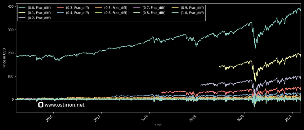
With a linear space and loop computation of the fractions, we can obtain the shape for each of the fractionally differentiated prices, with a default threshold value:

diffs = np.linspace(0,1,11).round(2)
plot_data = {}
for diff in diffs:
    plot_data[diff]  = standard_frac_diff(spy_close, diff)
    
p_data = pd.concat(plot_data, axis=1)
rh.plot_df(p_data)

It takes a little while to loop through the differentiation space, resulting in the familiar shapes for truncated fractionally differentiated time series:

The model sacrifices speed in the computation for easier handling of the returned data, so now we know where we are dropping values and can easily calculate the loss of information for each time series as we look for a stationary time series describing the movements of the price.

We are placing this implementation inside this Github repository. More features can be easily added to pre-process and inspect price series data before feeding it into machine learning models. We will slowly extend and properly package these particular implementations. The demonstration notebook is at the very end of the publication.

Information in ostirion.net does not constitute financial advice; we do not hold positions in any of the companies or assets that we mention in our posts at the time of posting. If you require quantitative model development, deployment, verification, or validation, do not hesitate and contact us. We will also be glad to help you with your machine learning or artificial intelligence challenges when applied to asset management, trading, or risk evaluations.

On the cover for this post: Phoenix fractal with constant 0.3333 made with online fractal generator.

The functions used in this post, as part of a notebook: